Portfolio Environment

PortfolioTradingEnv allocates a portfolio across N assets and cash. The agent outputs target weights, the env fills them at the close, values the book one bar later and charges fees and funding. N is read from the data.

Two classes share one money function, portfolio_step():

Class	Use it for	Bookkeeping
PortfolioTradingEnv	evaluation, baselines, LLM actors	history with values, weights, costs and turnover per step
VectorizedPortfolioTradingEnv	training (steps num_envs lanes at once)	rewards only

Their portfolio values match to 1e-9 on the same actions, so a policy trained on the vectorized env is evaluated faithfully on the scalar one.

from torchtrade.envs.offline import PortfolioTradingEnv, PortfolioTradingEnvConfig
from torchtrade.envs.offline.infrastructure.utils import load_portfolio_dataset

bars, instruments, funding = load_portfolio_dataset(revision="v2026.09")
config = PortfolioTradingEnvConfig(
    time_frames=["1Hour"], window_sizes=[50], execute_on="4Hour",
    transaction_fee=0.0005, allow_short=False,
)
env = PortfolioTradingEnv(bars, config, funding=funding)

Data

bars is long format, one row per asset and bar: timestamp (UTC, bar open), inst_id, open, high, low, close, volume, optional tradable. A missing row means the asset was not tradable at that bar; its last close is carried forward. Rows that stop before the end of the data mean the asset was delisted: the position is closed at its last tradable close. funding (optional) has timestamp, inst_id, funding_rate. Non-finite prices or rates are rejected.

Action, observation, timing

Action. Target weights [w_cash, w_1, ..., w_N]. The env normalises any vector to w_cash + Σ|w_i| = 1 with w_cash ≥ 0, clips shorts unless allow_short=True, and caps gross exposure at max_gross (≤ 1). Assets that are not tradable at the decision bar keep their holding; the rest of the budget follows the requested proportions.

Observation. portfolio_weights (N+1, drifted weights, cash first), tradable (N), and market_data_{tf}_{window} (N × window × 3: close, high, low divided by the window's latest close; zero before an asset lists).

Timing. The agent observes bars up to and including n, the rebalance fills at close n, and the step is valued at close n+1 with funding for settlements in (fill n, fill n+1]. A done env stepped before its reset re-emits its terminal transition with reward 0.

Costs and assumptions

• A trade pays transaction_fee × |notional traded| (a perpetual swap's fee). The post-trade value solves μ = 1 − fee·Σ|w'_i − μ·w_i| exactly. transaction_fee defaults to 0; set your venue's taker rate.
• Zero slippage and zero market impact: every trade fills at the close and does not move it.
• Funding is charged on the weights at the end of the step, which is exact when settlements fall on execute_on boundaries.
• No leverage: gross exposure is at most 1, and an unlevered book cannot be liquidated.

Baselines

Three baselines from the online portfolio selection literature live in torchtrade.actor. Each is a callable policy(td) -> td that writes td["action"], so it runs through env.rollout() exactly like a trained policy, on either env.

Baseline	Rule
UBAH()	Uniform buy and hold: equal weights once, then never rebalance
UCRP()	Uniform constant rebalanced portfolio: back to equal weights every step
OLMAR(window=5, epsilon=10.0)	On-line moving average reversion (Li & Hoi, 2012): bet on the window mean over the latest close

from torchtrade.actor import OLMAR, UBAH, UCRP
from torchtrade.metrics import portfolio_metrics

env.rollout(env.sampler.num_exec, policy=UCRP())
print(portfolio_metrics(env.history, periods_per_year=6 * 365))  # 4-hour bars

examples/offline/portfolio_baselines.py runs all three on Torch-Trade/okx-multi-asset-1h (40 perpetual swaps, 2026-03-12 to 2026-09-13, 1h bars, initial cash 10,000) at 1h, 4h and 1d decisions, at OKX's regular-tier taker fee of 0.05% with funding charged. These are the numbers an RL policy trained on this dataset has to beat, on the same window and frequency:

decisions	baseline	final value	Sharpe	max drawdown	turnover	commission	funding
1h	UBAH	1.206	1.16	−0.219	1.0	5	327
1h	UCRP	1.229	1.31	−0.186	16.3	89	285
1h	OLMAR	0.417	−1.14	−0.709	5506	18,456	234
4h	UBAH	1.211	1.22	−0.213	1.0	5	328
4h	UCRP	1.236	1.37	−0.180	8.7	48	287
4h	OLMAR	0.478	−0.95	−0.726	2004	6,187	211
1d	UBAH	1.192	1.09	−0.207	1.0	5	327
1d	UCRP	1.225	1.29	−0.172	4.5	24	285
1d	OLMAR	1.073	0.62	−0.540	337	2,339	386

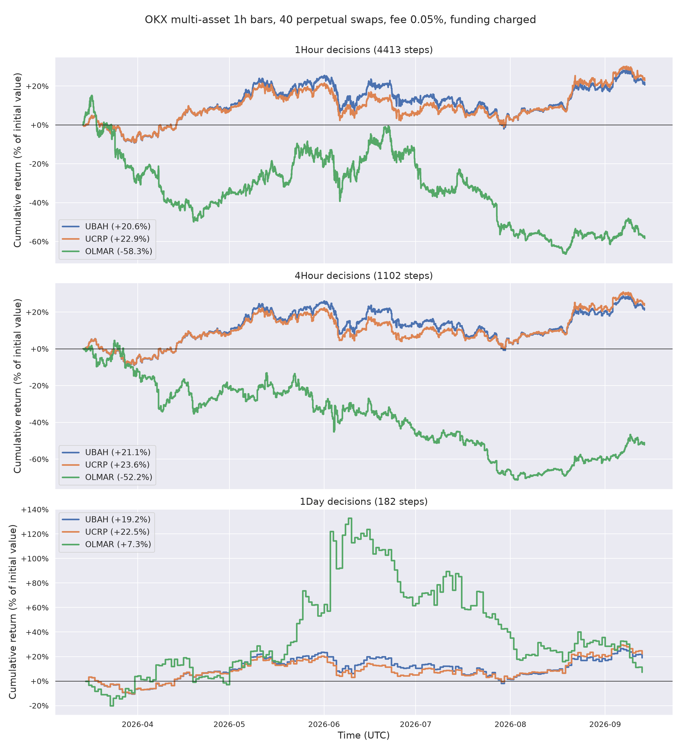
What to read off this. UCRP beats UBAH on every frequency with a shallower drawdown: selling what rose and buying what fell harvests the universe's volatility at a cost of a few dozen USD in commission. Funding, not commission, is the dominant cost of holding this universe (about 3% of initial value over six months). OLMAR turns the book over from 337x (1d) to 5,506x (1h); at zero fee it is the best strategy at 4h (1.30x), at the taker fee it loses half the account at 1h and 4h and keeps +7% at 1d with a 54% drawdown. Equal weight is the bar: a learned policy that does not beat UCRP after costs, on both final value and drawdown, has not learned anything the market did not hand it. The dataset's selection bias (below) lifts every one of these curves, and lifts a learned policy the same way.

Metrics

portfolio_metrics(history, periods_per_year) returns the standard metrics of compute_all_metrics (return, Sharpe, Sortino, Calmar, drawdown, win rate) plus final_value (p_f / p_0) and the episode totals of turnover (Σ|w_filled − w_drifted| over the assets, per step), commission and funding. The scalar env's history also exposes each of these per step through history.to_dict(). Like every offline env's history, it covers the current episode and starts over on reset(), so evaluate over the whole timeline as one episode (random_start=False, no max_traj_length), as the example does.

To compare your own policy, pass it to the same rollout:

env.rollout(env.sampler.num_exec, policy=my_policy)
metrics = portfolio_metrics(env.history, periods_per_year=6 * 365)

Dataset caveat

The 40 instruments in Torch-Trade/okx-multi-asset-1h were selected by liquidity measured at the end of the window, so backtests over that window carry selection bias. Choose the universe from data before the test window.